Constraining Cosmological Parameters with Type Ia Supernovae Part I

In this problem, we will use data from Type Ia supernovae to constrain cosmological parameters.

This problem is based on The Supernova Cosmology Project, which is one of the two research teams that first determined a positive cosmological constant using redshift data from Type Ia supernovae. The team took data taken from various telescopes, including the HST to measure the magnitude of various supernovae as a function of their redshift. This work led to the 1997 discovery of the fact that the expansion of the universe is actually accelerating. The same work eventually won the 2011 Nobel Prize and the 2015 Breakthrough Prize in Fundamental Physics.

We use data from the said project for our analysis. The dataset we will use is called the SCP Union2.1 compilation. The compilation has data from 833 supernovae, drawn from 19 datasets but only a certain number pass usability cuts so we are going to use a subset of those 833 supernovae.

You can download the dataset from http://supernova.lbl.gov/Union/. Download the dataset that says Union2.1 Compilation Magnitude vs. Redshift Table (for your own cosmology fitter). Study the dataset and answer the following question.

1. How many usable supernovae are in the SCP Union2.1 dataset?

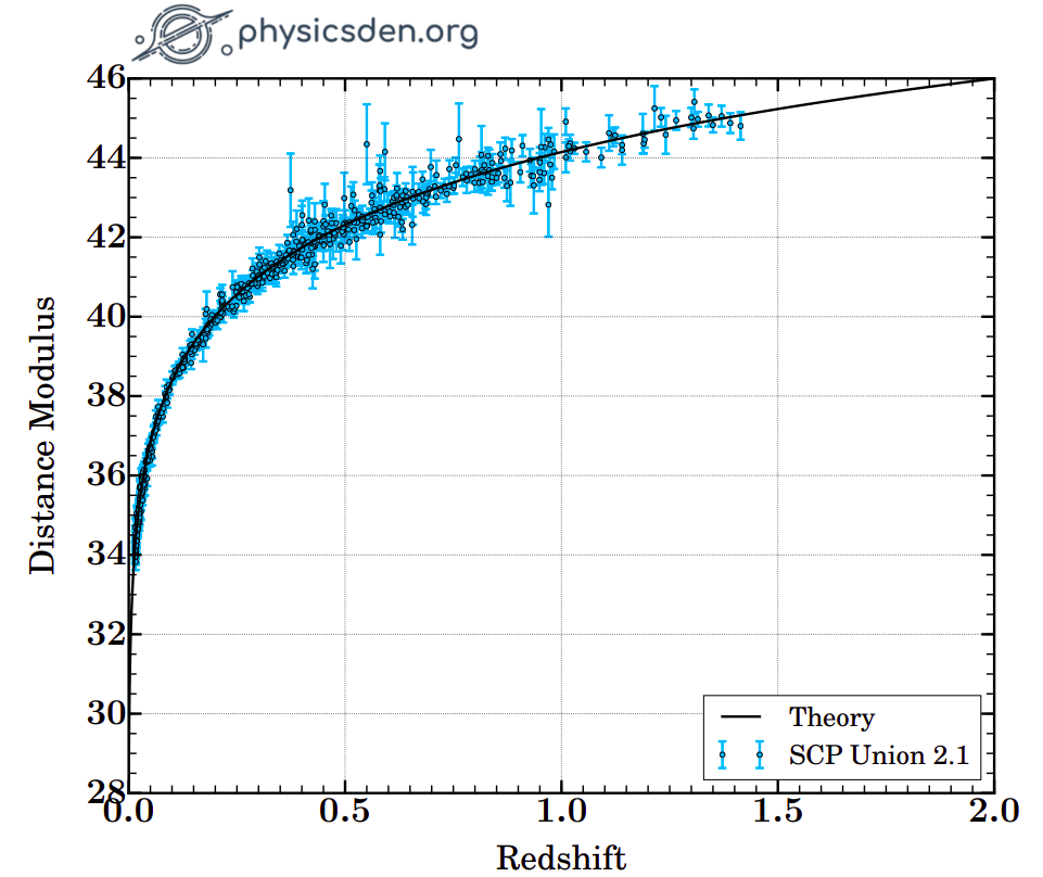
The columns are: supernova name, redshift, distance modulus, distance modulus error, and the probability that the supernova was hosted by a low-mass galaxy. Using this data, we can make what's called a Hubble diagram, which is a plot of distance against redshift.

Make the Hubble diagram with the given dataset. Your plot should look like the following.

The brightness of an object is measured by the apparent magnitude written in terms of the flux, $$m = -2.5 \log_{10}{\left( \frac{f}{f_x} \right)}$$ where $f_x$ is some normalization. In a similar fashion, the absolute magnitude is, $$M = -2.5 \log_{10}{\left( \frac{L}{L_x} \right)}$$ where $L_x$ is also some normalization. $f_x$ and $L_x$ are chosen such that the absolute magnitude corresponds to the apparent magnitude for a body 10 pc away. This makes the equation, $$m - M = 5 \log_{10}{\left( \frac{d_L}{10~\mathrm{pc}} \right)}$$ $$m= M + 5 \log_{10}{\left( \frac{d_L}{1~\mathrm{pc}} \right)} + 25$$ We can then write the magnitude $m$ as, $$ m = 5 \log_{10}\left( H_o d_L \right) + \mathcal{M} $$ $\mathcal{M}$ is a nuisance parameter that encodes uncertainties in the intrinsic luminosity and the Hubble constant. $d_L(z)$ is the luminosity distance and depends on the underlying cosmology and hence, in turn, $m$ depends on the cosmology. This means, if we have a measure of $m$, we can compare it to theoretical prediction of $m$ to test whether or not our universe supports the cosmology. $$m_{\mathrm{th}}(z, \left\{ p_j\right\}) = 5 \log_{10}{\left( \mathrm{H}_o \; d_L(z, \left\{ p_j \right\}) \right)} + \mathcal{M}$$ where $z$ is the redshift and $\left\{ p_j \right\}$ is the set of underlying cosmological parameters. The subscript th just means that this is the expected theoretical magnitude. Recall that $d_L(z)$ depends on the comoving distance $d_p(z)$ and $d_p(z)$ depends on the cosmological parameters as, $$ d_p(z) = \frac{c H_o^{-1}}{\sqrt{\left| \Omega_K \right|} } \mathrm{sinn} \left[ \sqrt{\left| \Omega_K \right|} \int_0^z \frac{\mathrm{d}z'}{\sqrt{ \Omega_M (1 + z')^3 + \Omega_\Lambda (1 + z')^{3(1 + w)} + \Omega_R (1 + z')^4 + \Omega_K(1 + z')^2 }} \right] $$ where "sinn(x)" is $\sinh{x}$, $\sin{x}$, or $x$ for an open, closed, and flat universe respectively, and $\Omega_K = 1 - \Omega_K - \Omega_R - \Omega_\Lambda$. This means $d_L(z)$ depends on the density parameters $\Omega$ and equation of state $w$. This dependence obviously then holds for $m$, allowing us to use the theoretical vs experimental values of $m$ to constrain those cosmological parameters. We will use maximum likelihood analysis to constrain our parameters. We can use $\chi^2$ value between data and theory to write our likelihood. In particular, $$ \chi^2 = ( {\bf m} - {\bf m}_{\mathrm{th}})^{\mathrm{T}} {\bf \mathrm{Cov}}^{-1} ( {\bf m} - {\bf m}_{\mathrm{th}}) $$ where $\bf \mathrm{Cov}$ is the covariance matrix. Then, the likelihood is just $$ \mathcal{L} = k \exp{\left( - \frac{\chi^2}{2} \right)} $$ where $k$ is a normalization factor. The normalization isn't super important but choosing it such that $\mathcal{L}$ is bounded by $1$ would allow an interpretation in terms of probability.

We can now write a Python function for our likelihood.

def calculate_likelihood(chi2):
    # Implement the function here.
    return likelihood

We're going to need the theoretical values of magnitude $m_{\mathrm{th}}$ so let's implement it but before that we need to implement the luminosity distance $d_L$. The luminosity distance depends on the comoving distance $d_{\mathrm{comov.}}$, which would in turn depend on the redshift $z$, equation of state $w$, and density parameters $\Omega_M$ and $\Omega_{\lambda}$. Implement this function and answer the questions below to check your implementation.

c = 299792  # Speed of light in km/s
H0 = 70 # Hubble constant
M = 25 # Nuisance parameter


def comoving_distance(z, w=-1, Omega_M=1.0, Omega_L=1.0):
    # Implement the function here.

def luminosity_distance(z, w, Omega_M, Omega_L):
    # Implement the function here.
    return d_L

def m_th(z, w, Omega_M, Omega_L):
    # Implement the function here. 
    # Calculate d_L with the function luminosity_distance() above.
    return likelihood

2. What is comoving_distance(z=0.5, w=-1, Omega_M=0.25, Omega_L=0.75)? Answer to 1 decimal place.

3. What is luminosity_distance(z=0.5, w=-1, Omega_M=0.25, Omega_L=0.75)? Answer to 1 decimal place.

4. What is m_th(z=0.5, w=-1, Omega_M=0.25, Omega_L=0.75)? Answer to 1 decimal place.

For this problem, we will ignore the covariance matrix and assume it to be the identity matrix. The Union2.1 website does provide the covariance matrix if you want to use it to go beyond this problem.

We now have all the ingredients we need. We have the experimental measures of $m$ that we can calculate with the downloaded luminosity distances. We can now also calculate the theoretical values of $m$. With these two sets of information, we can vary our parameter values while looking at how that affects the likelihood. We want to maximize the likelihood, which would be equivalent to minimizing the $\chi^2$ value.

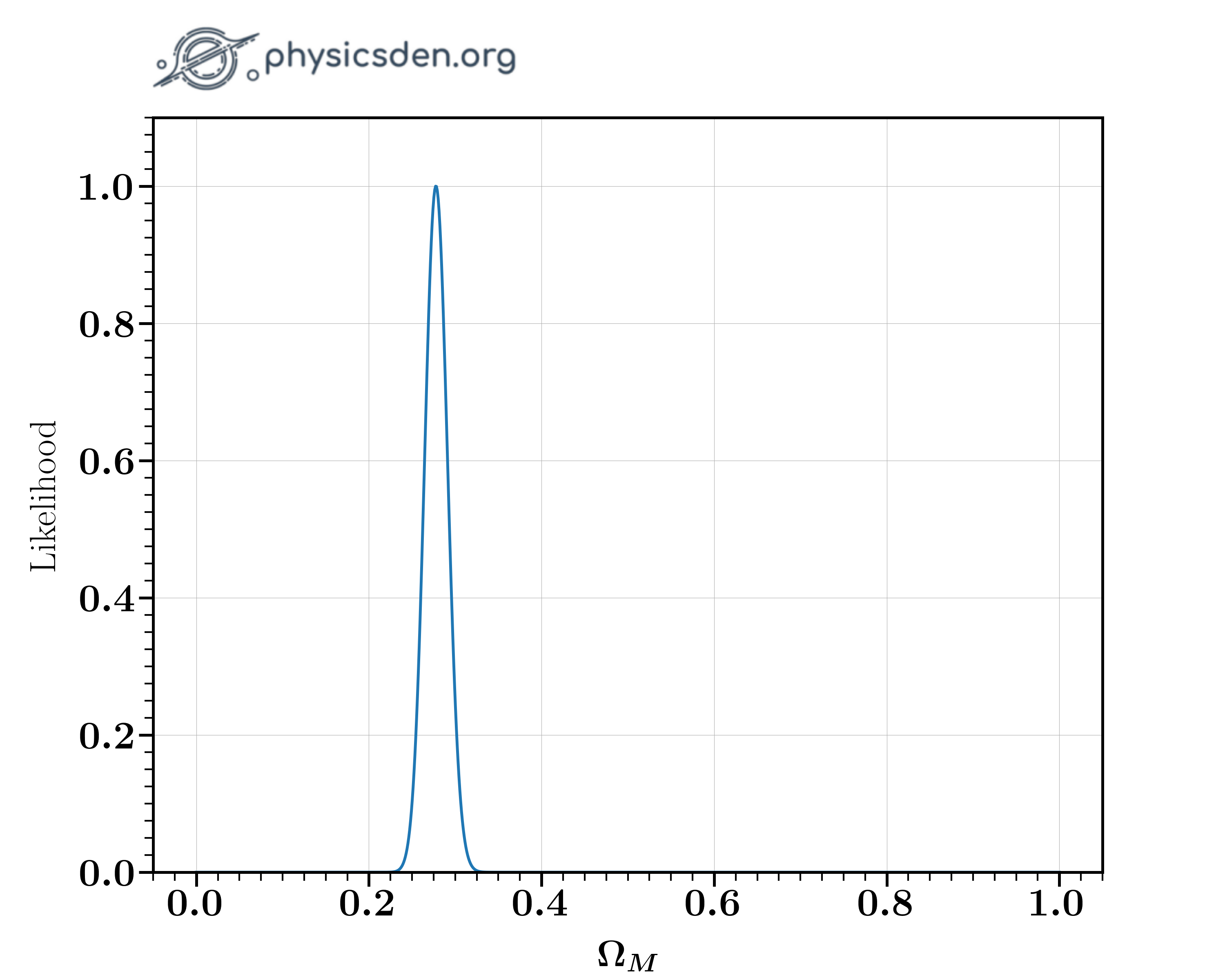
For this optimization, we need to calculate the $\chi^2$ values, so let's write a function to do so. Complete the code with hints given below. This should let you find the $\Omega_M$ value that maximizes the likelihood. You could also plot the likelihood as a function of $\Omega_M$. Your result should look like the image below.

def calculate_chi2(data, params):
    z_s, mag_s, errors = data
    omega_M, omega_DE, w = params

    # Calculate chi2.

    return chi2

def search_for_Omega_m():

    z_s, mag_s, errors = load_data("SCPUnion2.1_mu_vs_z.txt")
    w = -1
    omega_M_s = np.linspace(0, 1, 1000)
    
    # Calculate likelihoods.

    # Find Omega_M that gives maximum likelihood.

5. What $\Omega_M$ gives you the maximum likelihood? Answer to 1 decimal place.

Now that we found the most likely value of $\Omega_M$, let's do a similar maximization to find constraints on two parameters simultaneously. In particular, let's optimize $\Omega_M, w$, and $\Omega_M, \Omega_{\Lambda}$.

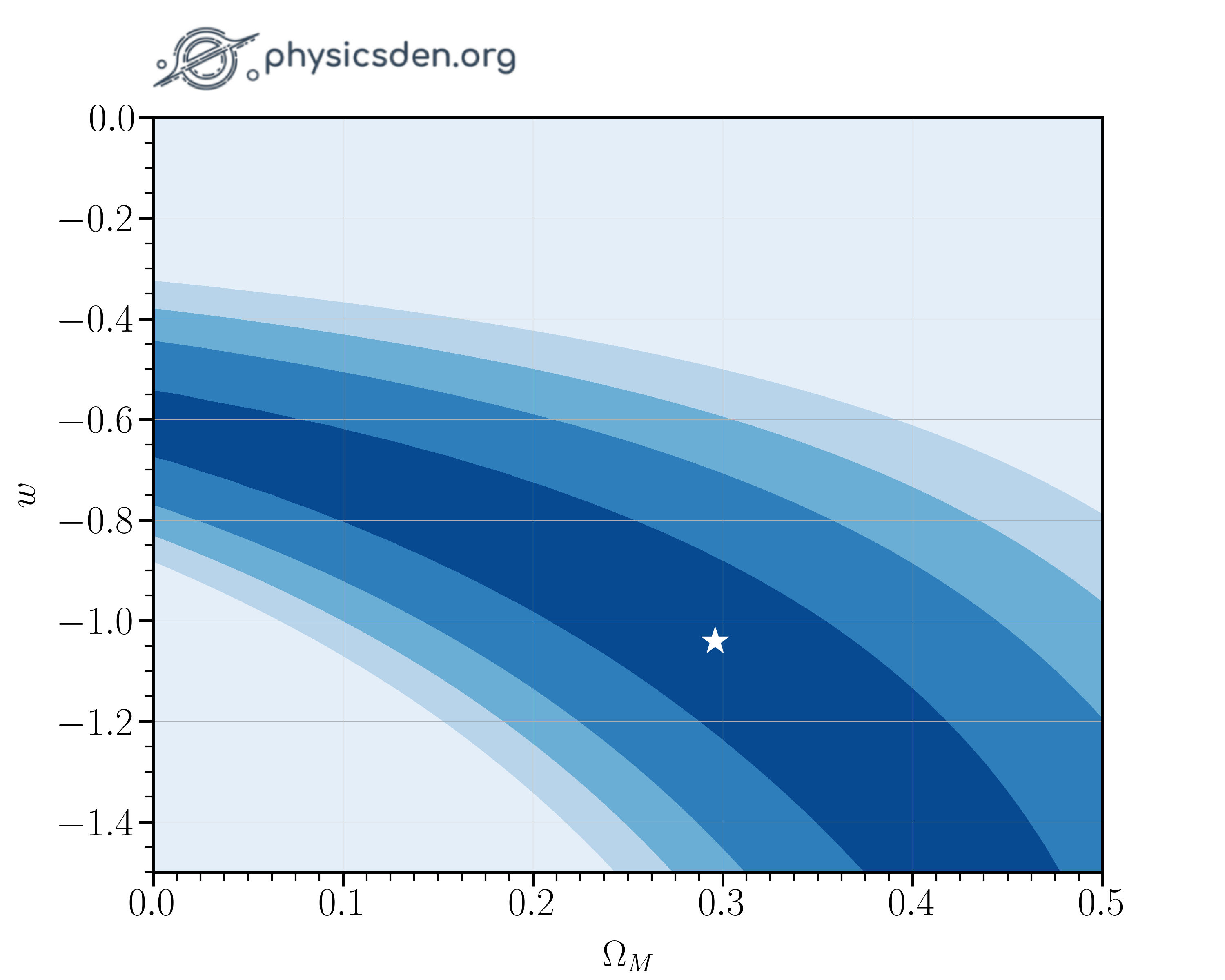
Create a 2d grid of prospective parameter values and use that to maximize the likelihood. Fill in the code below to find the most likely values for $\Omega_M$ and $w$.

def search_for_Omega_m_and_w():

    z_s, mag_s, errors = load_data("SCPUnion2.1_mu_vs_z.txt")

    N = 50
    
    omega_M_s = np.linspace(0, 0.5, N)
    w_s = np.linspace(-1.5, 0, N)

    likelihood_s = np.zeros((N, N))

    # Loop through omega_M and w_s and find the optimum likelihood.

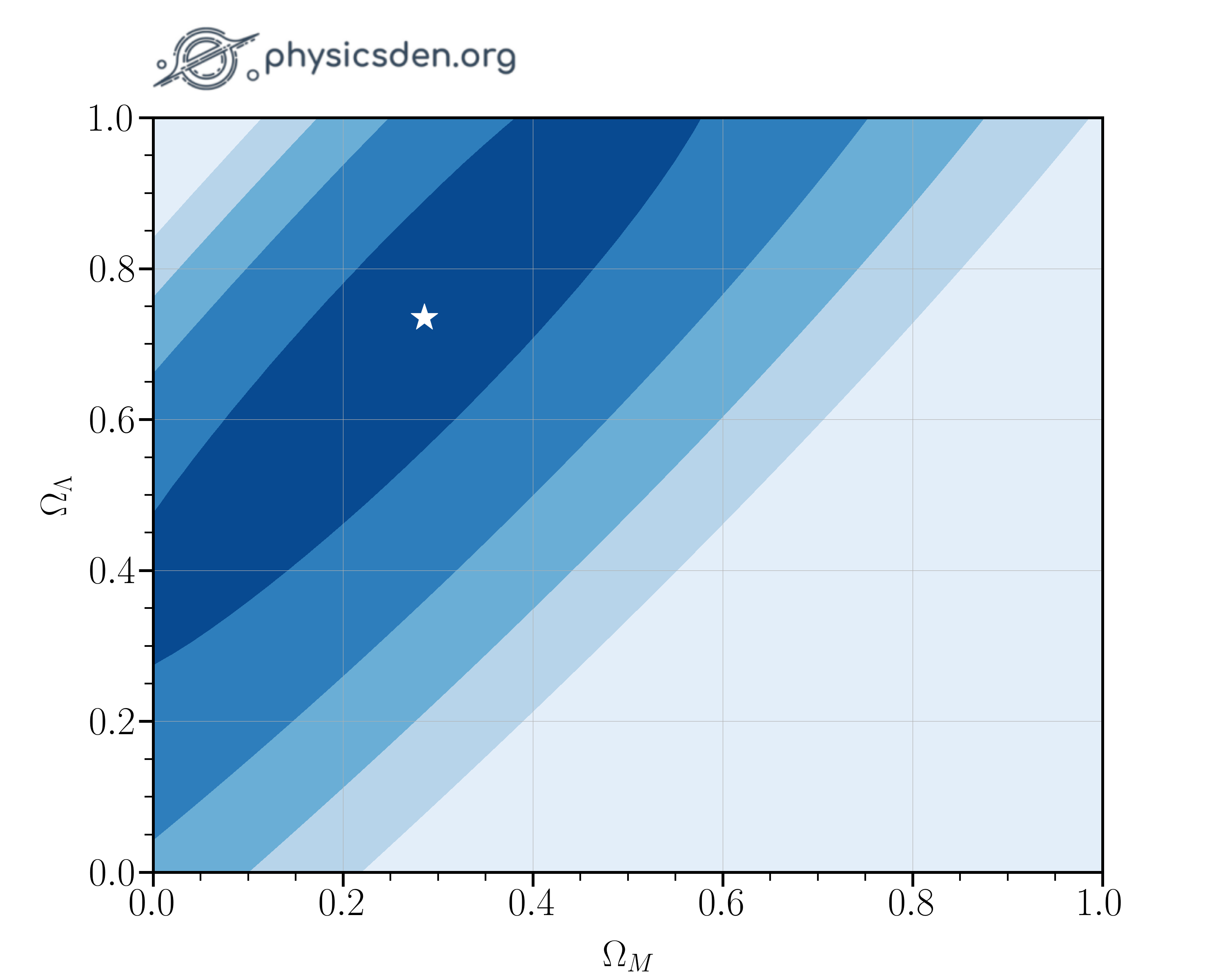
If you make a 2D contour plot of your likelihood, it should look something like the images below.

6. What is the optimum $\Omega_M$? Answer to 1 decimal place.

7. What is the optimum $w$? Answer to 1 decimal place.

Repeat the steps you just took to find the most likely values for $\Omega_M$ and $\Omega_{\Lambda}$ simultaneously.

def search_for_Omega_m_and_Omega_L():

    N = 50
    
    omega_L_s = np.linspace(0.0, 1.0, N)
    omega_M_s = np.linspace(0.0, 1.0, N)

    likelihood_s = np.zeros((N, N))

    # Loop through omega_M and omega_L and find the optimum likelihood.

8. What is the optimum $\Omega_M$? Answer to 1 decimal place.

9. What is the optimum $\Omega_{\Lambda}$? Answer to 1 decimal place.

You used data from Type Ia supernovae to constrain cosmological parameters $\Omega_M, \Omega_{\Lambda}, w$. This was an example of using maximum likelihood to compare experimental data with a theoretical model and using that for inference on unknown parameters. When you have a large number of parameters, it is inefficient to do a grid search like we did here. A common approach for such situations is to use Markov Chain Monte Carlo (MCMC) to find the set of parameters that maximizes the likelihood. We will explore MCMC in a future problem.