Temperature Anisotropies in the CMB Map Part I

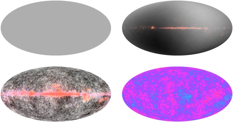
In this problem, we investigate the temperature anisotropies in the CMB map. The CMB temperature is constant everywhere up to 1 part in 100. This constant temperature map corresponds to a monopole. In other words, the monopole is the "average" of the map. If we go a step further, there is a dipole in the map. A dipole is a pattern of a hot region on one side and a cold region on another side. This dipole is a consequence of the Earth's motion around the solar system, the solar system's motion around the galaxy, and so on. As we move across the universe, the CMB temperature is red-shifted in a region and blue-shifted in the opposite region, producing a dipole in the map. Information about this dipole can be used to accurately calculate our position and velocity with respect to the CMB rest frame.

For the purpose of finding out more cosmological information, we can remove the dipole and further enhance the contrast of the CMB map. When this is done, increasing the contrast to the level of 1 in 100,000, the map shown in the bottom-left corner of Fig. 1 is obtained. The feature in the equator is contamination from our galaxy, which has been removed in the bottom-right corner of the figure. This “noisy” looking map shows quantum fluctuations in the early universe. These are the early seeds that eventually led to the formation of structure in the universe.

Similar to how we can decompose functions into Fourier series, we can decompose angular functions into a series of spherical harmonics. Click here and here to learn more about spherical harmonics. This is known as the multipole decomposition. We can write,

$$ \frac{\delta T}{T} (\theta, \phi) = \sum_{\ell=\ell_o}^{\infty} \sum_{m = -\ell}^{m = +\ell} a_{\ell m}Y_{lm} $$ where the coefficients are, $$ a_{\ell m} = \int \frac{\delta T}{T} Y_{\ell m}^{*} (\theta, \phi) \, \mathrm{d} \Omega \,. $$

1. What is the minimum value of $\ell$ we use in the decomposition above, $\ell_o$? Remember that the monopole represents no anisotropies and the dipole term corresponds to our "cosmic movement".

Studying the coefficients of the spherical harmonics, $a_{\ell m}$ gives us a direct window to the physics of the early universe as that is where the temperature anisotropies come from.

Working with spherical harmonics allows us to separate scales and map a relation between $\ell$ and the corresponding angular scale $\theta$. Each $\ell$ corresponds to characteristic variations on the scale of $$ \theta \simeq \frac{\pi}{\ell} = \frac{180^o}{\ell} \, . $$

Inflation predicts that these temperature variations are Gaussian. If inflation is correct, this means the coefficients $a_{\ell m}$ can be completely characterized just by their variance (the mean of the Gaussian being zero) [arXiv:astro-ph/0210603]. This provides a way to write $a_{\ell m}$ in terms of their variance $C_{\ell}$. Notice that while $a_{\ell m}$ has both an $\ell$ and $m$ index, the variance $C_{\ell}$ depends only on $\ell$. This comes from statistical isotropy- the variation in the azimuthal direction is constant so we do not need to specify a value for $m$.

It is convenient to write the power spectrum as $\ell (\ell + 1) \frac{C_{\ell}}{2\pi}$ so we define $D_l= \ell (\ell + 1) \frac{C_{\ell}}{2\pi}$. We often call this the angular power spectrum.

As a warmup, we will use data from WMAP and PLANCK experiments to calculate the angular power spectrum i.e. make a plot of $D_{\ell}$ vs. $\ell$.

Begin by downloading the required data files. WMAP data can be downloaded from here. For this part of the problem, go to TT Power Spectra and download the file called "Seven Year Combined TT Power Spectrum" (click here to learn more about CMB polarization). Open the file in your favorite text-editor and explore around a little bit to see what kinds of data the file has and how you can use it to compute $D_{\ell}$.

Now, make a plot of $D_{\ell}$ against $\ell$ using just the WMAP data. Next, we'll add results from the PLANCK data to it.

For PLANCK data, go here. Under Public Release 2, go to Ancillary Data. Then, click on Power Spectrum and download the given COM_PowerSpect_CMB_R2.02.fits file. Also take a look at the accompanying header file. It will be important in a little bit.

As you might have noticed, PLANCK data is in a weird format called a FITS file. So we need to do a little bit of work to get our $D_{\ell}$ values out. We are going to use Astropy to work with FITS files. Install Astropy in your computer. Information about working with FITS files can be found here. You can use the following skeleton code as your starting point. Note that the file you downloaded contains 12 BINTABLE extensions. This essentially means that there are 12 different data tables in there. More information about what those tables are can be found in the download page here. We are interested in the "TT" power spectrum. The power spectrum for $\ell$ of 2 to 29 is the table called TTLOLUNB. Note its index from the webpage above. Next, we want the power spectrum for higher values of $\ell$. This is TTHILUNB. Notice its index too.

from astropy.io import fits
from astropy.table import Table

# Do stuff here.

data_low_l = fits.getdata(filename, index_of_low_l_table)
data_low_l_table = Table(data_low_l)
print data_low_l_table

# Do stuff here.

data_high_l = fits.getdata(filename, index_of_high_l_table)
data_high_l_table = Table(data_high_l)
print data_high_l_table

# Do more stuff here.

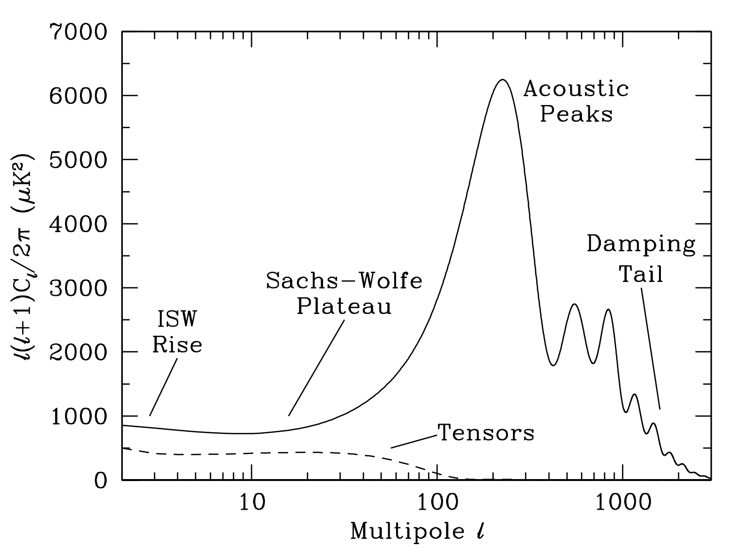
Plot the power spectrum for $\ell$ between 2 to 1200. Make both a linear and log x-scale version. The log-version should look like the following.

If your plot also looks like this, congratulations, you have successfully completed part I of this problem. Stay tuned for the second part.

If you are interested to read more about the features of the plot and how it tells us enormous information about the early universe, check out these slides. This paper is also really helpful. More information about the acoustic peaks can be found here. Also check out Professor Wayne Hu's tutorials here. You're also more than welcome to use the forum here to ask questions about any of this.